How Search Engines Work: Base Search and Inverted Index
Under the hood of almost every search omnibox the same fiery heart beats, named a search engine. It is a search engine that takes words and returns a list of relevant documents to the user.
The article describes the structure of a search engine and its optimizations with references to theory. Tantivy, a Rust implementation of the Lucene architecture, is used as a test subject. The article turned out to be concentrated, mathematical, and incompatible with relaxed reading with a cup of coffee, beware!
The formal problem setting: there is a set of text documents, and we want to be capable to
- quickly find the most relevant documents in this set based on the text query
- add new documents to the set for subsequent search.
At the first step, we will define what document relevance to the query is, and we will do it in a way that is suitable to a computer. At the second step, we will find a top-K of the most relevant documents and show them to the user. And then we will make everything work with a nice performance.
Definition of Relevance
Relevance in human language means the semantic proximity of a document to a query. In mathematical language, proximity can be expressed through the proximity of vectors. Therefore, for the mathematical expression of relevance, it is necessary to associate vectors in some vector space with documents and queries from the world of people.
Then, a document will be considered relevant to a query if the document-vector and the query-vector are close in the vector space. A search model with such a definition of proximity is called a vector search model.
The main issue with the vector search model is how to construct the vector space \(V\) and to transform documents and queries into \(V\). In general, vector spaces and transformations can be any as long as closely related documents and queries are mapped to close vectors.
Modern libraries allow to build complex vector spaces with a small number of dimensions and dense information content in each dimension with just a few clicks. In such spaces all vector coordinates characterize particular aspect of the document or query: theme, mood, length, lexicon, or any combination of these aspects. Often, coordinate value cannot be explained in human language, but is understood by machines. A simple plan for building such a search is:
- Take your favorite library for building text embeddings, such as fastText or BERT, and transform the documents into vectors
- Store the obtained vectors in your favorite K nearest neighbors (k-NN) search library, such as faiss
- Transform the search query into a vector using the same method as for documents
- Find the nearest vectors to the query vector and extract the corresponding documents
A k-NN based search will be very slow, especially if you try to index and search over the entire Internet. So, we narrow down the definition of relevance to make it computationally feasible.
Note: Here and onwards “words” in the context of documents and queries will be referred as “terms” to avoid confusion
Let’s represent relevance as two mathematical functions and then fill them with meaning:
- \(score(q, d)\) - the relevance of the document to the query
- \(score(t, d)\) - the relevance of the document to one term
We impose the restriction of additivity on \(score(q, d)\) and express the relevance of the query through the sum of its terms’ relevance: \(score(q, d)=\sum_{t \in q}score(t, d)\)
Additivity simplifies further computations, but forces us to agree with a strong simplification of reality - as if all words in the text occur independently of each other.
The most well-known additive relevance functions are TF-IDF and BM25. They are used in most search systems as ones of the main relevance metrics.
The origin of TF-IDF and BM25
If you know how to derive the formulas from the title, you can skip this part.
Both TF-IDF and BM25 measure the relevance of a document to a query with a single number. Higher values of the metrics mean that the document is more relevant. The values themselves do not have any meaning per se. But by comparing of metric values we may find more relevant documents to the query, ones that have bigger values.
Let’s try to repeat the reasoning of the formulas’ authors and reproduce the steps of building TF-IDF and BM25. We will denote the number of indexed documents as \(N\). The simplest thing to do is to define relevance equal to the number of occurrences of the term (term frequency or \(tf\)) in the document:
\[score(t, d)=tf(t, d)\]If we have not a single term \(t\), but a query \(q\) consisting of several terms, and we want to calculate \(score(q, d)\) for this document, what should we do? We remember the constraint of additivity and simply sum up all the separate \(score(t, d)\) for the terms from the query:
\[score(q, d)=\sum_{t \in q}score(t, d)\]We have an issue with the above formula because we do not take into account the different “importance” of different terms. If we have a query “cat and dog”, then the most relevant documents will be those that contain 100500 occurrences of the term “and”. It is unlikely this is what the user wants to get.
Let’s fix the issue by weighing each term according to its importance: \(score(t, d)=\frac{tf(t, d)}{df(t)}\) where \(df(t)\) is the number of documents containing term \(t\). It turns out that more frequent terms are less important and \(score(t, d)\) becomes smaller. Terms such as “and” will have a huge \(df(t)\) and therefore a small \(score(t, d)\).
Seems better already, but now we have another issues - the \(df(t)\) has no any intrinsic meaning. If \(df(giraffe) = 100\), and \(N\) equals to 100, then the term “giraffe” is considered very frequent in this case. But if \(N\) equals to 100 000, then it seems too rare.
The dependence of \(df(t)\) on \(N\) can be eliminated by transforming \(df(t)\) into a relative frequency with dividing by \(N\):
\[score(t, d)=\frac{tf(t, d)}{\frac{df(t)}{N}}=tf(t, d)\frac{N}{df(t)}\]Now let’s assume we have 100 documents, one contains “elephant,” two others contains “giraffe”. \(\frac{N}{df(t)}\) in the first case will be equal to 100, and in the second - 50. The term “giraffe” will receive two times fewer points than the term “elephant” just because there are one more document with giraffe than with elephants. We are going to fix it by smoothing the function \(\frac{N}{df(t)}\).
Smoothing can be performed in different ways, we will do this by taking the logarithm:
\[score(t, d) = tf(t, d)\log\frac{N}{df(t)}\]We just got TF-IDF. Let’s move on to BM25.
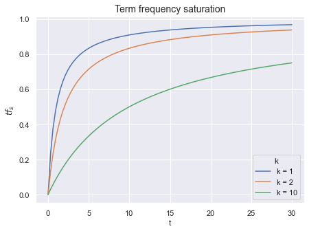
It is unlikely that a document containing the term “giraffe” 200 times is twice as good as a document containing the term “giraffe” 100 times. So let’s smooth things out again, but now not by logarithm, but a little differently. Replace \(tf(t, d)\) with
\[tf_s(t, d) = \frac{tf(t, d)}{tf(t, d) + k}\]With each increase in the number of term occurrences \(tf(t, d)\) by one, the value of \(tf_s(t, d)\) grows smaller and smaller - the function is smoothed out. And with the parameter \(k\) we can control the curvature of this smoothing. Speaking smarter, the parameter \(k\) controls the degree of saturation of the function.
The function \(tf_s(t, d)\) has two remarkable side effects.
Firstly, \(score(q, d)\) will be greater for documents that contain all the words in the query than for documents that contain only one word from the query multiple times. The top-K of documents will be more pleasing to the user’s eyes this way.
Secondly, the value of the function \(tf_s(t, d)\) is upper bounded. The rest of \(score(t, d)\) is also upper bounded, so the whole function \(score(t, d)\) is upper bounded (further the upper bound value will be named as \(UB_t\)). Moreover, \(UB_t\) is very easy to calculate in our case.
Why is \(UB_t\) important for us? \(UB_t\) is the maximum possible contribution of this term to the relevance of entire query. If we know \(UB_t\), we can cut corners during executing the query.
The final step is to start taking into account the lengths of documents in \(score(t, d)\). In long documents, the term “giraffe” may appear simply by chance and its presence in the text tells nothing about the real topic of the document. But if a document consists of one term and this term is “giraffe”, then we can confidently assert that the document is about giraffes.
The obvious way to take into account the length of the document is to put the number of document words \(dl(d)\) into the formula.
Additionally, we would like to divide \(dl(d)\) by the average number of words in all documents \(dl_{avg}\) for normalization, due to the same reasons as for \(df(t)\) above: better to use relative values instead of absolute ones.
Now let’s find a place for the document length in our formula. When \(k\) grows, \(tf_s\) decreases. If we multiply \(k\) by \(\frac{dl(d)}{dl_{avg}}\), it turns out that longer documents will receive a lower \(score(t, d)\). That’s what we need!
It is possible to further parameterize the impact of the document length to the overall score. Let’s replace \(\frac{dl(d)}{dl_{avg}}\) with \(1 - b + b\frac{dl(d)}{dl_{avg}}\) and obtain:
\[\frac{tf_s(t, d)}{tf_s(t, d) + k(1 - b + b\frac{dl(d)}{dl_{avg}})}\]When \(b = 0\), the formula may be simplified into \(\frac{tf_s(t, d)}{tf_s(t, d) + k}\), and when \(b = 1\), the formula takes the form
\[\frac{tf_s(t, d)}{tf_s(t, d) + k\frac{dl(d)}{dl_{avg}}}\]Once again, \(k\) is the impact of the repeating terms on relevance, and \(b\) is the impact of the document length on relevance.
Let’s substitute \(tf\) into \(tf_s\):
\[score(q, d)=\sum_{t \in q} \frac{tf(t, d) (k + 1)}{tf(t, d) + k(1 - b + b\frac{dl(d)}{dl_{avg}})} * \log\frac{N}{df(t)}\]We have obtained the BM25 formula with a minor nuance. In the canonical formula \(\log\frac{N}{df(t)}\) (this term is called \(IDF\)) is replaced by \(\log\frac{N - df(t) + 0.5}{df(t) + 0.5}\). This substitution is based on fitting to a theoretically purer form of the RSJ model and does not have simple heuristics behind it. This form of \(IDF\) gives a lower weight to terms that appear too often: articles, conjunctions, and other letter combinations that carry little information.
An important note: from the BM25 formula it is now evident that \(UB_t\) is more dependent on the frequency of the term in the corpus. The less frequent the term, the higher its maximum possible contribution to \(score(q, d)\).
Implementation of Inverted Index
Given the limited memory, slow disks, and processors, we now need to design a data structure capable of producing the top-K BM25 relevant documents.
We have a set of documents, and we want to search in them. All documents are assigned a document ID or DID. Each document is divided into terms, terms can be truncated or converted to a canonical form if desired. For each processed term, we create a list of documents (precisely, documents’ DIDs) containing this term is created. The name of such list is a posting list.

Different implementations of inverted indexes may also store the exact places of term in a document or the total number of term occurrences. This additional information is used in calculating relevance metrics or for executing specific queries where the mutual arrangement of terms in the document is important (such as phrase queries). The posting list itself is sorted in ascending order of DID, although there are other approaches to its organization.
The second part of the inverted index is a term dictionary. A KV store is used for the dictionary, where terms are the keys and values are the addresses of posting lists in RAM or on disk. Hash tables and trees are usually used for the KV store in memory. However, other structures may be more appropriate for the term dictionary, such as prefix trees.

In Tantivy, finite-state transducers are used by default for term storage through the fst crate. Simplifying it, prefix trees organize the dictionary by extracting common prefixes of the keys, while transducers can also extract common suffixes. Thus, the compression of the dictionary is performed more efficiently, but in the end, it becomes an acyclic graph instead of a tree.
The fst library can compress even better than general-purpose compression algorithms in extreme cases while still preserving arbitrary access. Extreme cases occur when a large portion of your terms have long common parts. For example, when you store URLs in an inverted index.
The fst library also has serialization and deserialization methods for the dictionary, which greatly simplifies life - storing trees and graphs by hand on disk is still entertainment. Unlike hash tables, fst allows wildcard substitution during key searches. Some people reportedly use the asterisk in search queries, but I haven’t seen any.
Another option for storing the dictionary is SSTable. It is just a delta-compressed blocks of keys, possibly with secondary indices. The performance of SSTables is worse than fst, but search in SSTables require less of random memory accesses. This property may be especially beneficial in network-mapped dictionaries.
Using a term dictionary and posting lists, one can determine a list of documents for a single term \(t\). Then it remains to calculate \(score(t, d)\) for each document from the posting list and take the top-K documents.
To do this, we will look how \(score(t, d)\) can be implemented in the computer world.
In Tantivy, BM25 is used as one of the options for a relevance function:
\[score(t, d)=\sum_{t \in q} \frac{tf(t, d) (k + 1)}{tf(t, d) + k(1 - b + b\frac{dl(d)}{dl_{avg}})} * \log\frac{N - df(t) + 0.5}{df(t) + 0.5}\]- \(tf(t, d)\) - we calculate the number of occurrences of document DID in the posting list of term \(t\), or store it as a separate number, which will speed up the entire process by using additional memory
- \(df(t)\) - length of the entire posting list
- \(dl_{avg}\) - calculated based on two statistics, the total number of documents in the index and the total length of all posting lists. Both statistics are kept by the inverted index actual after adding a new document
- \(dl(d)\) - stored for each document in a separate list
In addition to the term dictionary, posting lists and document lengths, Tantivy (and Lucene) saves in files:
- Exact word positions in documents
- Skip-lists for acceleration iteration through lists (read further)
- Direct indexes, which allow extracting documents by its DID. Direct indexes may be slow because documents are usually compressed using heavy codecs like brotli
- FastFields - a KV storage built into the inverted index. It can be used to keep arbitrary values, for example external statistics of a document such as PageRank. These values may be used then in calculating custom \(score(q, d)\) functions
Now, we know how to calculate \(score(q, d)\) for a one-term query and need to find the top-K documents. The first idea is to calculate the scores for all documents, sort in descending order and take the first K. It spends a lot of RAM, and with a large number of documents, we’ll run out of memory.
Fortunately, we know what is Top-K heap and may use it. In details, the first K documents are placed unconditionally in a heap, and then each subsequent document is first evaluated and placed in the heap only if its \(score(q, d)\) is higher than the minimum \(score(q, d)\) from the heap.
Queries with Multiple Terms
What will an inverted index do with the query “download OR cats”? It will create two iterators on the posting lists for the terms “download” and “cats”, start iteration on both lists, calculating \(score(q, d)\) while iterating and maintaining a top-K heap. Similarly, an AND-query is implemented, however here iteration allows for skipping significant parts of the posting lists without calculating \(score(q, d)\) for them.
OR-queries are more important for general-purpose search engines because they cover more documents and because ranking queries with metrics like TF-IDF or BM25 still raises documents with a higher number of matching words to the top of the list. This makes the top-K documents more similar to the result of an AND-query.
The naive implementation of an OR query algorithm is as follows:
- Create iterators for the posting lists of each term in the query
- Initiate a top-K heap
- Sort the iterators (not the contents of the posting lists, but the set of iterators) by the DID they are currently pointing to
- Take the document that the first iterator is pointing to and gather among the remaining iterators those that point to the same document. This way we get the DID and the terms that are contained in the document
- Calculate the relevance of the document by the terms, sum them up, get the relevance for the entire query. If the document is good, then put it in the top-K heap
- Advance the used iterators and return to step 3

In step 4, the collection of iterators is carried out quickly since the list of iterators is sorted by DID. The reordering of iterators in step 3 can also be optimized if we know which iterators were advanced in step 6.
Some Optimizations in the Inverted Index
During typical search session, a user does not need all relevant documents, but only K most relevant ones. This opens the way for important optimizations. The reasoning of all optimization is simple - most of the documents will become unnecessary, and we may avoid overhead of iterating or calculating metrics over them.
Let’s take a closer look at the pseudocode of the OR algorithm Bortnikov, 2017:
Input:
  termsArray - Array of query terms
  k - Number of results to retrieve
Init:
  for t ∈ termsArray do t.init()
  heap.init(k)
  θ ← 0
  Sort(termsArray)
Loop:
  while (termsArray[0].doc() < ∞) do
    d ← termsArray[0].doc()
    i ← 1
    while (i < numTerms ∩ termArray[i].doc() = d) do
      i ← i + 1
    score ← Score(d, termsArray[0..i − 1]))
    if (score ≥ θ) then
      θ ← heap.insert(d, score)
    advanceTerms(termsArray[0..i − 1])
    Sort(termsArray)
Output: return heap.toSortedArray()

function advanceTerms(termsArray[0..pTerm])
  for (t ∈ termsArray[0..pTerm]) do
    if (t.doc() ≤ termsArray[pTerm].doc()) then
      t.next()
The naive algorithm has an \(O(LQ\log{Q})\) asymptotic behavior, where L is the total length of the posting lists used in processing the query, and Q is the number of words in the query. It can be slightly improved by eliminating \(Q\log{Q}\), as most users bring queries no longer than some maximum and \(Q\log{Q}\) can be considered a constant.
In practice, the performance of the inverted index mostly depends on the size of the corpus (i.e., the total length of the posting lists) and the frequency of requests. Request auto-completion or internal analytical requests in a search system can significantly multiply the system load. Even \(O(L)\) becomes too grim estimate.
Compression of Posting Lists
The size of the posting lists can reach gigabytes. Storing posting lists as they are and traversing them entirely is a bad idea. The main reason is the more you need to read from the disk, the slower everything works. Therefore, posting lists are the first candidates for compression.
Let’s recall that a posting-list is an increasing list of unsigned integers (DIDs). The numbers in the posting-list are not significantly different from each other and lie in a relatively limited range of values from 0 to some number comparable to the number of documents in the corpus.
VarLen Encoding
Spending 8 or 4 bytes of fixed integers to encode a small number is a waste. So people came up with codes that represent small numbers using a small number of bytes. Such schemes are called variable length encodings. We will be interested in a specific scheme known as varint.
Reading a number in varint is done byte by byte. Each read byte stores a signal bit and 7 bits of payload. The signal bit tells us whether we need to continue reading or if the current byte is the last for this number. The payload is concatenated until the last byte of the number.
Posting lists can be compressed well with varint by several times, but now our hands are tied - we can’t jump forward in the posting list by N numbers, because it is unclear where the boundaries of each DID are. It turns out that we can only read the posting list sequentially, and there is no way for parallel reads now.
SIMD
To allow parallel reading, trade-off schemes similar to varint were invented. In such schemes, numbers are divided into groups of N numbers and each number in the group is encoded with the same number of bits, and the whole group is preceded by a descriptor that describes what is in the group and how to unpack it. The same length of packed numbers in a group allows using SIMD instructions (SSE3 in Intel) for unpacking groups, which speeds up our performance.
Tantivy packs DIDs into blocks of 128 numbers, and then writes a block of 128 term frequencies using bitpack encoding.
Delta-encoding
Varint compresses small numbers well and compresses large numbers worse. In the posting list we have only increasing numbers, hence the compression quality will become worse when new documents are added. But let’s store not DIDs themselves, but the difference between the neighboring DIDs. For example, instead of [2, 4, 6, 9, 13] we will store [2, 2, 2, 3, 4].
The list of constantly increasing numbers will turn into a list of small non-negative numbers. Such a list can be compressed more efficiently, but now decoding the i-th number requires summing of all numbers up to the i-th. However, this is not a big deal, because varint scheme assumes that reading is sequential anyway.
Skip-lists for iterating through posting lists
After compressing posting lists become something like linked lists. All we can do is to traverse the list from start to end. You may think we haven’t needed more, but the optimization schemes described in the following sections require the ability to move iterators forward by an arbitrary number of DIDs and sequential forwarding starts to appear too slow.
No wonder we have a nice decision here named skip-lists. Skip-list is a sparse index for the list of number. If you want to find X in the list of numbers, the skip-list will explain to you in \(O(log(L))\) time what is the position in the original list approximately before X. After the jump, you should go up to X with a regular linear search.
The precision of the jump depends on the amount of memory we can allocate for the skip-list, which is a typical trade-off in algorithms. In Tantivy, movement along the posting-list is implemented using skip-lists.
In our skip-list implementation, we also need to store partial sums up to the point where we plan to jump. Otherwise, delta encoding won’t allow us to decode the original number.
Optimizing OR Queries
All optimizations of posting list traversal can be divided into safe and unsafe. As a result of applying safe optimizations, the top-K documents remain unchanged compared to the naive OR algorithm. Unsafe optimizations can give a big speed gain, but they change top-K and may miss some documents.
MaxScore
MaxScore is one of the first known attempts to speed up the execution of OR-queries. The optimization is safe and described in Turtle, 1995.
The essence of the optimization is to split the query terms into two non-intersecting sets: “mandatory” and “optional”. Documents that contain terms only from the “optional” set cannot enter the top-K and therefore their posting lists can be skipped forward to the first document that contains at least one “mandatory” term.
Remember the \(UB_t\) term introduced in the section on TF-IDF and BM25? I remind you that this is a someway “importance” of the term. Common words have low importance, and specific words have high importance. \(UB_t\) is a function of the frequency of the term and can be calculated on the fly based on the size of the posting list.
Having the importance of terms at hand, one can sort all the terms from the query in decreasing order of their importance and calculate the partial sums of importance from the first to the last term. All terms with a partial sum less than the current \(\theta\) (the current minimum score from the top-K heap) can be assigned to the “optional” set. A document containing only terms from the “optional” set cannot be rated higher than the sum of the importance of these terms and therefore cannot be rated higher than \(\theta\). Such documents will not be included in the final set.
Makes sense to consider documents that contain at least one term from the “mandatory” set of terms only. Therefore, we can skip the posting lists of “optional” terms until the smallest of the DIDs that the “mandatory” term iterators point to. Without skip-lists we would have to run through the posting lists sequentially and there would be no big gain in speed.

After each update of the top-K heap, the two sets are rebuilt, and the algorithm terminates when all terms end up in the “optional” set.
Weak AND (WAND)
WAND is also a safe search optimization method described in Broder, 2003, which is similar to MaxScore in that it analyzes partial sums \(UB_t\) and \(\theta\).
- All WAND term iterators are sorted in the order of DID, which each iterator points to
- The partial sums of \(UB_t\) are calculated
- The pivotTerm is selected - the first term whose partial sum exceeds \(\theta\)
- All previous iterators to the pivotTerm are checked. If they point to the same document, then that document may theoretically be part of the top-K documents, and therefore a full calculation of \(score(q, d)\) is performed for it. If at least one of the iterators points to a DID less than pivotTerm.DID, then such an iterator is advanced to a DID greater than pivotTerm.DID. After that, we return to the first step of the algorithm
Block-max WAND (BMW)
BMW is an extension of the WAND algorithm from the previous section, proposed in Ding, 2011. Instead of using global \(UB_t\) for each term, we now split the posting lists into blocks and store \(UB\) separately for each block. The algorithm repeats WAND, but also checks the partial sum of \(UB\) of the blocks that the iterators are currently pointing to. If this sum is below \(\theta\), the blocks are skipped.
Block-level \(UB\) estimates of terms are much lower in most cases than global \(UB_t\). As a result, many blocks will be skipped and this will save time in calculating the \(score(q, d)\) of documents.
To understand the gap between production inverted indexes and academic research, you can delve into the ticket LUCENE-4100.
Block Upper Scoring
Alongside the \(UB\) for a block, other metrics can be stored to help make the decision not to touch this block. Or, adjust the \(UB\) itself in the right way so that its value reflects your intent.
The author of the article experimented with a search where only fresh news documents were required. BM25 was replaced with \(BM25D(q, d, time) = BM25(q, d) * tp(time)\) where \(tp\) is a function that imposes a penalty on outdated documents and takes values from 0 to 1. By changing the formula for \(UB\), it was possible to pass 95% of all blocks with outdated news, which significantly speeded up this particular search.
Preprocessing of the Search Query
Before the query lands to an inverted index, it undergoes several stages of processing.
Query Parsing

First, the query syntax tree is built. Punctuation is discarded from the query, the text is converted to lowercase, tokenized, and stemming, lemmatization, and stop-word elimination may be used. Further, a logical tree of operations is built from the token stream.
Whether tokens are joined by default with the OR or AND operator depends on the index settings. On one hand, connecting through AND can sometimes give a more accurate result, on the other hand, there is a risk of finding nothing at all. Although, you may produce several queries, and after their execution, choose the best one based on the size of the result or external metrics.
The logical tree is the basis for the executing plan. In Tantivy, the corresponding structure is called a Scorer. The Scorer implementation is the center of the inverted index universe because this structure is responsible for iterating over posting lists and for all possible optimizations of this process.
Query Expansion Stage
Almost always, users want to receive not what they are requesting, but something slightly different. And therefore, large search engines have complex systems trying to guess what you want and expand your request with additional terms and constructions.
The query is diluted with synonyms, different weights are attributed to terms. Search engine may use a history of previous searches, add filters, use the search context and a million other hacks. This stage of work is called query extension, and it is incredibly important for improving search quality.
It is cheap to conduct experiments as this stage. Imagine that you want to find out if using morphology in a search will give you any profit. Morphology in this context is the conversion of different word forms to the canonical form (lemma).
For example:
download, downloaded, downloading -> download
cats, kitty, cat -> cat
You have several options:
- Heavy: Try to modify an inverted index source code for storing both lemmas and word forms. A lot of programming and documents re-indexing is required
- Trade-off: Re-index documents with converting all word forms to lemmas on the fly. Less programming, but still requires re-indexing
- Simple: Just add all word forms to the query. In this case, the user’s query “download cats” will be transformed into something like “(download^2 OR downloaded OR downloading) AND (cats^2 OR kitties OR cat OR kitty)”. No re-indexing is needed!
In the simple approach, all hypothetical processor costs for re-indexing will be transferred to the query extension stage and to the execution stage. This may save you a lot of time. Fail often, fail fast.
Index Recording and Segmentation
In the Lucene architecture, the inverted index is divided into segments. A segment stores its portion of documents and is immutable. To add documents, we collect new documents in RAM, make a commit, and at this point, the documents from RAM are saved to a new segment.
Segments are immutable because data associated with the segment (skip lists or sorted posting lists) is also immutable. It is not possible to quickly add data to them, as this would require a complete rebuilding of the data structure.
Segments can process queries simultaneously, so the segment is the natural unit of load balancing. The complexity arises only in merging results from different segments, as an N-Way Merge of document streams from each segment must be performed.
However, many small segments are bad. This sometimes happens when we record data in small portions. In such situations, Tantivy launches a segment merging procedure, turning many small segments into one big segment.
During segment merging, some data, such as compressed documents, can be quickly merged, while other structures are rebuilt, and it loads your CPU. So the schedule of merges strongly affects the overall index performance under constant write load.
Sharding
There are two ways to parallelize the load on the inverted index: by documents or by terms.
In the first case, each of the N servers stores only a portion of the documents, but is a standalone mini-index. In the second, it stores only a portion of the terms for all documents. The answers from the shards in the second case require additional non-trivial processing.
| By Documents | By Terms | |
|---|---|---|
| Network Load | Small | Large |
| Storing Additional Attributes for Document | Easy | Difficult |
| Disk-seeks for Query from K words on N shards | O(K*N) | O(K) |
Usually, network load is a bigger problem than disk work. That’s why Google used document-based splitting in its early indexes. It is also more convenient to use document-based sharding in Tantivy - the segments of the index are natural shards.
Since segment rebuilding in an inverted index is a heavy operation, it is better to immediately start using Ring or Jump Consistent Hashing schemes to reduce the volume of documents to be re-sharded upon opening a new shard.
Multiphase Search and Ranking
In search systems, two parts are usually distinguished: base searches and meta-searches. Base search makes queries one corpus of documents. Meta search makes queries to several base searches and cleverly merges the results of each base search into a single list.
Base searches can be conditionally divided into one- and two-phase searches. The above article describes a one-phase search. Such a search ranks the list of documents with computationally simple metrics such as BM25, using a variety of optimizations, and returns documents to the user without serious postprocessing.
The first phase of two-phase (or even multiphase) searches does the same thing. But in the second phase, the top-K documents from the first phase are re-ranked using computationally heavier metrics.
In practice, part of the complex metrics of the second phase often grow into the first phase over time and allow for immediate correction of relevance and posting list traversal to improve the quality of the final result.
First Ranking Phase
The document-to-query matching metric can be very simple, such as \(BM25\), or slightly more complex, such as \(BM25 * f(IMP)\), where \(IMP\) is the static quality of the document, and \(f\) is an arbitrary mapping with values belonging to \([0; 1]\).
The restriction on \(f\) in this case arises from the optimizations used in the BMW-type index, which do not allow modifying \(score(t, d)\) without changing the saved block \(UB\).
BM25 is calculated during the work with the posting lists, and additional members like \(IMP\) should be stored next to the inverted index. This is the first significant limitation of the first search phase. Through the function \(score(q, d)\), in general, too many documents are processed for it to be possible to run for each of them to some external systems for additional document attributes.
In web search, the role of the \(IMP\) member is usually performed by PageRank, calculated once every N days on large MapReduce clusters. The calculated PageRank is written to a fast KV-storage of an inverted index, such as FastFields in the case of Tantivy, and is used in the calculation of relevance.
Documents from other sources may have other metrics. For example, for search in scientific articles, it makes sense to use the impact factor or citation index.
Second phase of ranking
In the second phase of ranking, you have more room for applying complex metrics. You have hundreds to thousands of more or less relevant documents obtained from the first phase. The remaining time before the request deadline (usually fractions of a second) can be used to run machine learning, load metrics from external databases, and reorder documents to make the output even more relevant.
Retrieve click information from your statistical database and use user preferences to create a personalized output. You can even calculate something on the fly, such as a new version of BM25 or whatever you want.
This stage of work is one of the most engaging in search development and also important for good output quality.
Search Quality
Search quality control deserves a separate article, here I will just leave a couple of links and give a few practical tips.
The main goal of quality control is testing and monitoring the results of releasing new versions of the index. Any quality metric should be an approximation of user satisfaction to some extent. Keep this in mind when inventing something new.
At the initial stage of search development, any increase in the quality metric usually means a real improvement in search quality. But the closer you are to the upper limit of the theoretically possible quality, the more diverse artifacts will arise when optimizing a certain metric.
You will need a lot of logs. To calculate search quality metrics, it is necessary to store the following information for each user query: the list of DID search results and the values of their relevance function in the current search session, DID and positions of clicked documents, user interaction times with the search, and session identifiers. Weights that characterize the quality of the session can also be stored. This way, it is possible to exclude robot sessions and give greater weights to sessions of assessors (if you have them).
Next, a couple of metrics to start with. They can easily be formulated even in terms of SQL queries, especially if you have something like Clickhouse for storing logs.
Success Rate
The first and most obvious one - did the user find anything at all within the session.
with 1.959964 as z
select
    t,
    round(success_rt + z*z/(2*cnt_sess) - z*sqrt((success_rt*(1 - success_rt) + z*z/(4*cnt_sess))/cnt_sess)/(1 + z*z/cnt_sess), 5) as success_rate__lower,
    round(success_rt, 5) as success_rate,
    round(success_rt + z*z/(2*cnt_sess) + z*sqrt((success_rt*(1 - success_rt) + z*z/(4*cnt_sess))/cnt_sess)/(1 + z*z/cnt_sess), 5) as success_rate__upper
from (
    select
        toDateTime(toDate(min_event_datetime)) as event_datetime,
        $timeSeries as t,
        count(*) as cnt_sess,
        avg(success) as success_rt
    from (
        select
            user_id,
            session_id,
            min(event_datetime) as min_event_datetime,
            max(if($yourConditionForClickEvent, 1, 0)) as success
        from
            $table
        where
            $timeFilter and
            $yourConditionForSearchEvent
        group by
            user_id,
            session_id
    )
    group by
        t,
        event_datetime
)
order by
      t
MAP@k
A good introduction to MAP@k and several other learning-to-rank metrics can be found on Habr. The metric characterizes how good your top-K documents are, where K is usually taken equal to the number of elements on the search results page.
select
    $timeSeries as t,
    avg(if(AP_10 is null, 0, AP_10)) as MAP_10
from
(
    select
        session_id,
        min(event_datetime) as event_datetime
    from (
        select
            session_id,
            event_datetime
        from
            query_log
        where
            $timeFilter and
            $yourConditionForSearchEvent
    )
    group by
        session_id
) search
left join
(
    select
        session_id,
        sum(if(position_rank.1 <= 10, position_rank.2 / position_rank.1, 0))/10 as AP_10
    from (
        select
            session_id,
            groupArray(toUInt32(position + 1)) as position_array_unsorted,
            arrayDistinct(position_array_unsorted) as position_array_distinct,
            arraySort(position_array_distinct) as position_array,
            arrayEnumerate(position_array) as rank_array,
            arrayZip(position_array, rank_array) as position_rank_array,
            arrayJoin(position_rank_array) as position_rank
        from
            query_log
        where
            $timeFilter and
            $yourConditionForClickEvent
        group by
            session_id
    )
    group by
        session_id
) click
on
    search.session_id = click.session_id
group by
    t
order by
    t
Instead of Conclusion: Google and their First Inverted Index

Sergei Brin and Larry Page created the first version of Google and indexed about 24 million documents in 1998. The students implemented document downloading using Python, running a total of 3-4 spider processes. One spider processed about 50 documents per second. The full database was filled in 9 days, and it required hundreds of GB of data to be downloaded. The index took tens of disk GB.
Google invented its own architecture of an inverted index, different from the one that will be used a year later in the first versions of Lucene. The format of the Google index was as simple as 50 cents and, in my opinion, very beautiful.
The foundation of the index is Barrel format files. A Barrel is a text file that stores quadruples ⟨did, tid, offset, info⟩, sorted by ⟨did, offset⟩. In this notation, did is the document ID, tid is the term ID, and offset is the position of the term in the document.
In the original system, there were 64 such Barrel files, each of which was responsible for its own range of terms (tid). A new document received a new did and the corresponding quadruples were added to the end of the Barrel files.
A set of such Barrel files is a direct index that allows you to retrieve a list of terms for a given did with a binary search on did (the files are sorted by did). The inverted index can be obtained from the direct index by the operation of inverting - we take and sort all files by ⟨tid, did⟩.

Done! Now binary search can be used to search by tid.
The format of Barrel files clearly shows the traces of MapReduce concepts, fully realized and documented in the work J.Dean, 2004.
There is a lot of good readings about Google in the public domain. You can start with the original work Brin, 1998 about the search architecture, then dive into the lectures of the New Jersey Institute of Technology, and polish everything off with a presentation by J.Dean on the Google’s internals.
Imagine you come to work and they tell you that for the whole next year, you’ll need to speed up the code by 20% each month to stay afloat. That’s how Google lived in the early 2000s. Developers at the company had ended up with forcibly relocating index files to external cylinders of hard disk drives because their linear rotation speed was higher and files were read faster.
Fortunately, in 2023 such optimizations are no longer necessary. HDDs are virtually replaced from operational work and the index, starting from the mid-2010s, is fully stored in RAM.
Further reading:
- The anatomy of a large-scale hypertextual Web search engine Brin, 1998
- PISA Project Documentation
- Как работают поисковые системы @iseg
- Compression, SIMD, and Postings Lists Trotman, 2014
- Query evaluation: Strategies and optimizations Turtle, 1995
- Efficient query evaluation using a two-level retrieval process Broder, 2003
- Faster top-k document retrieval using block-max indexes Ding, 2011